Poisson Distribution

A discrete, non-negative probability distribution that can be right skewed.

The Poisson distribution is used to model counts. If events counted within a fixed time are truly independent, then the Poisson distribution is not an approximation, but the probability distribution of counts.

In reality, counts are often not completely independent: Birds do not arrive randomly, independently in a park, but actually tend to group together. For this reason, analyses based on a Poisson distribution should include some assessment of whether the chosen distribution is realistic. These assessments will be introduced once we get to the topic of GLM.

Properties

What is the probability of a given count \(k\)?

Figure 1: Probability mass function of a Poisson distribution with \(\lambda = 3\).

Mathematical formula:

\[\begin{align} \tag{1}\label{dpois} \frac{\lambda^k e^{-\lambda}}{k!} \end{align}\]

Code:

R
Python

dpois(k, lambda)

from scipy.stats import poisson
poisson.pmf(k, mu)

Note: mu refers to the mean (\(\lambda\)).

Symbols

\(\lambda\): The rate parameter, representing both mean and variance
\(e\): The constant 2.718282… (why?)
\(k\): The value of a given count
\(!\): Factorial (e.g., \(3! = 3 \times 2 \times 1\))

Explanation

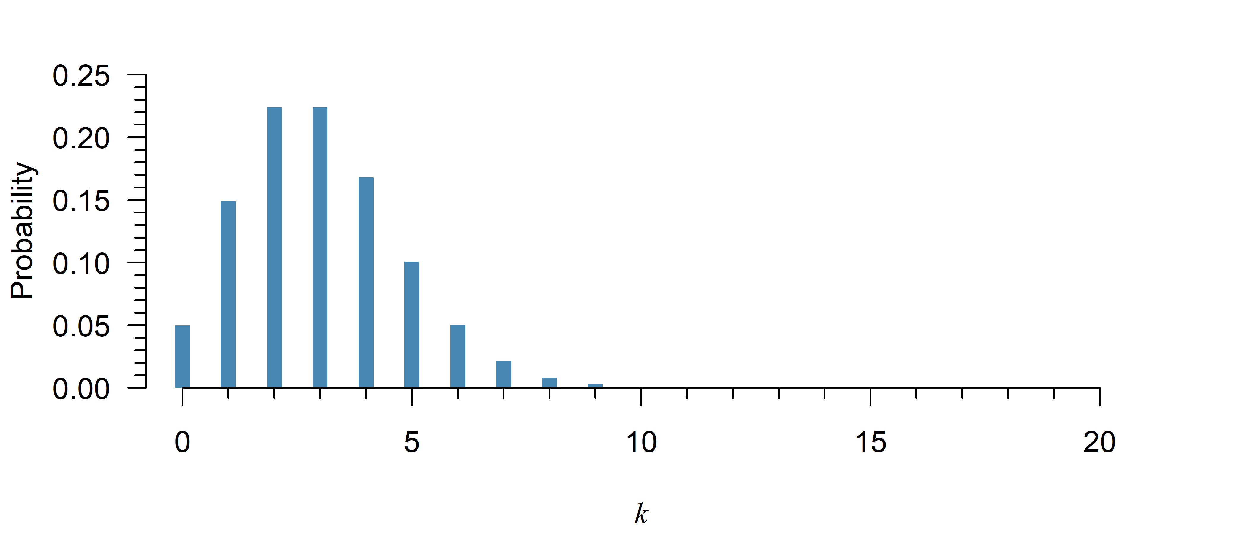
The Poisson distribution is a discrete probability distribution. There are only certain possible values for the outcome, like \(0, 1, 2, \dots\), but not \(1.5\) or \(2.01\). Hence, you can directly read probabilities off the \(y\)-axis in Figure 1.

The correct term for a probability function of a discrete distribution is a probability mass function, though it is common in literature to see people call both discrete and continuous versions a probability density function.

Note that while it looks like the probability goes to zero after \(k = 10\) in Figure 1, it never exactly reaches zero. The probability is just too small to be visible in the figure.

Example

R
Python

The probability of \(k = 4\) in Figure 1 is:

dpois(4, lambda = 3)

[1] 0.1680314

The probability of \(k = 4\) in Figure 1 is:

from scipy.stats import poisson
poisson.pmf(4, mu = 3)

0.16803135574154085

What is the probability up till a given point \(k\)?

Figure 2: Cumulative distribution function of a Poisson distribution with \(\lambda = 3\).

Mathematical formula:

\[\begin{align} \tag{2}\label{ppois} \sum_{i = 0}^k \frac{\lambda^i e^{-\lambda}}{i!} \end{align}\]

Code:

R
Python

ppois(k, mean, sd)

from scipy.stats import poisson
poisson.cdf(k, mu)

Note: mu refers to the rate \(\lambda\).

Symbols

\(\lambda\): The rate parameter, representing both mean and variance
\(e\): The constant 2.718282… (why?)
\(k\): The value of a given count
\(!\): Factorial (e.g., \(3! = 3 \times 2 \times 1\))
\(\sum\): Summation (compute for \(0, 1, \dots, k\) and add all results)

Explanation

The cumulative distribution function (CDF) is the sum of the probability mass function up till a given point \(k\). It can be used to calculate the probability of a count being no greater than a certain value. To obtain the opposite—the chance of an observation greater than a certain value, simply use \(1\) minus the CDF. Finally, to compute the chance of being within a certain range, you can subtract the CDF of the larger value, from the CDF of the smaller value (see the examples below).

Examples

R
Python

If there are on average 5 falling stars in the sky every night, the chance of observing no more than 3 on a given night is equal to:

ppois(3, lambda = 5)

[1] 0.2650259

And the chance of observing at least 3 is equal to:

1 - ppois(2, lambda = 5)

[1] 0.875348

(This works because you start with 1 (100%) exclude all options resulting in less than 3.)

To compute the probability of a certain range, just subtract the smaller value from the greater:

# Probability of 2 to 4 falling stars:
ppois(4, lambda = 5) - ppois(1, lambda = 5)

[1] 0.4000656

(This works because you start with all possibilities up till 4 and then exclude all options resulting in less than 2.)

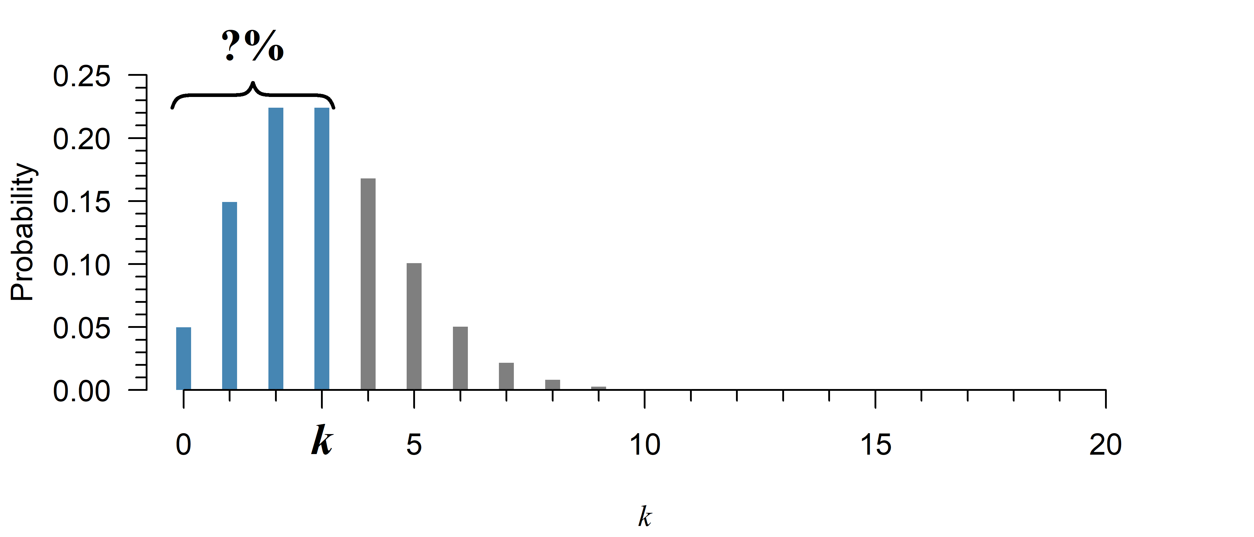
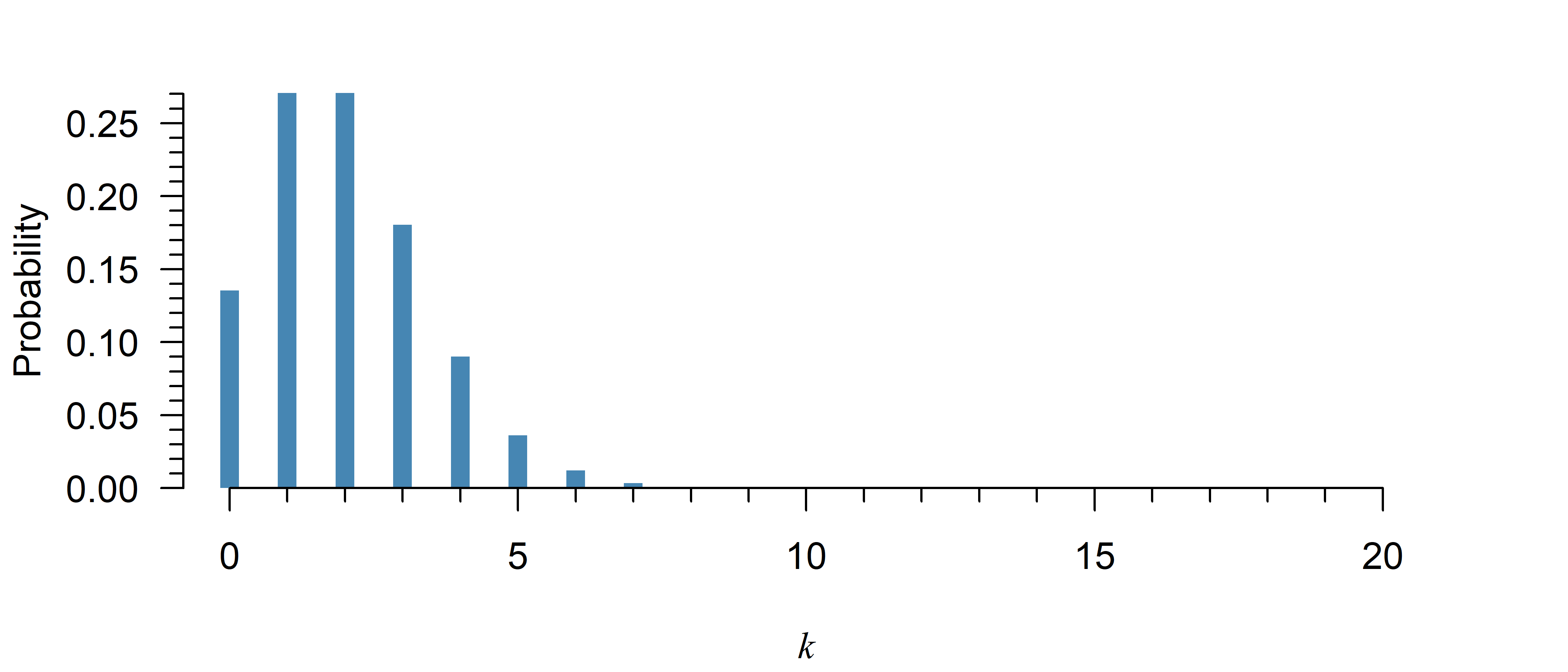
The probability of a value of \(k \leq 3\) in Figure 2 is given by:

ppois(3, lambda = 3)

[1] 0.6472319

If there are on average 5 falling stars in the sky every night, the chance of observing no more than 3 on a given night is equal to:

from scipy.stats import poisson
poisson.cdf(3, 5)

0.2650259152973616

And the chance of observing at least 3 is equal to:

1 - poisson.cdf(2, 5)

0.8753479805169189

(This works because you start with 1 (100%) exclude all options resulting in less than 3.)

To compute the probability of a certain range, just subtract the smaller value from the greater:

# Probability of 2 to 4 falling stars:
poisson.cdf(4, 5) - poisson.cdf(1, 5)

0.40006560307069977

(This works because you start with all possibilities up till 4 and then exclude all options resulting in less than 2.)

The probability of a value of \(k \leq 3\) in Figure 2 is given by:

poisson.cdf(3, 3)

0.6472318887822313

Up till what point does the probability equal at least \(p\)?

Figure 3: Quantile function of a Poisson distribution with \(\lambda= 3\).

Mathematical formula:

\[\begin{align} \tag{3}\label{qpois} \text{no simple closed form} \end{align}\]

Code:

R
Python

qpois(probability, lambda)

from scipy.stats import poisson
poisson.ppf(probability, mu)

Note: mu refers to the mean (\(\lambda\)).

Explanation

The quantile function is the inverse of the cumulative distribution function. It tells you up till what point the probability equals \(p\). To obtain the opposite—the point after which the probability equals a certain value, simply compute the quantile of \(1\) minus the probability (see the examples below).

There exists no simple expression for the quantile function of the Poisson distribution, but it can be computed anyway using a numeric search. If you are interested how this works, I explain it below.

If no simple closed form exists, how is it calculated?

The quantile function answers the opposite of the cumulative distribution function:

Cumulative distribution function: What is the probability \(p\) up till a certain count \(k\)?
Quantile function: What is the count \(k\) that has a probability of at least \(p\)?

This should give you a hint of how a numeric search might work: If you don’t have a quantile function, you can simply try plugging different \(k\)s in the cumulative distribution until you find the right answer.

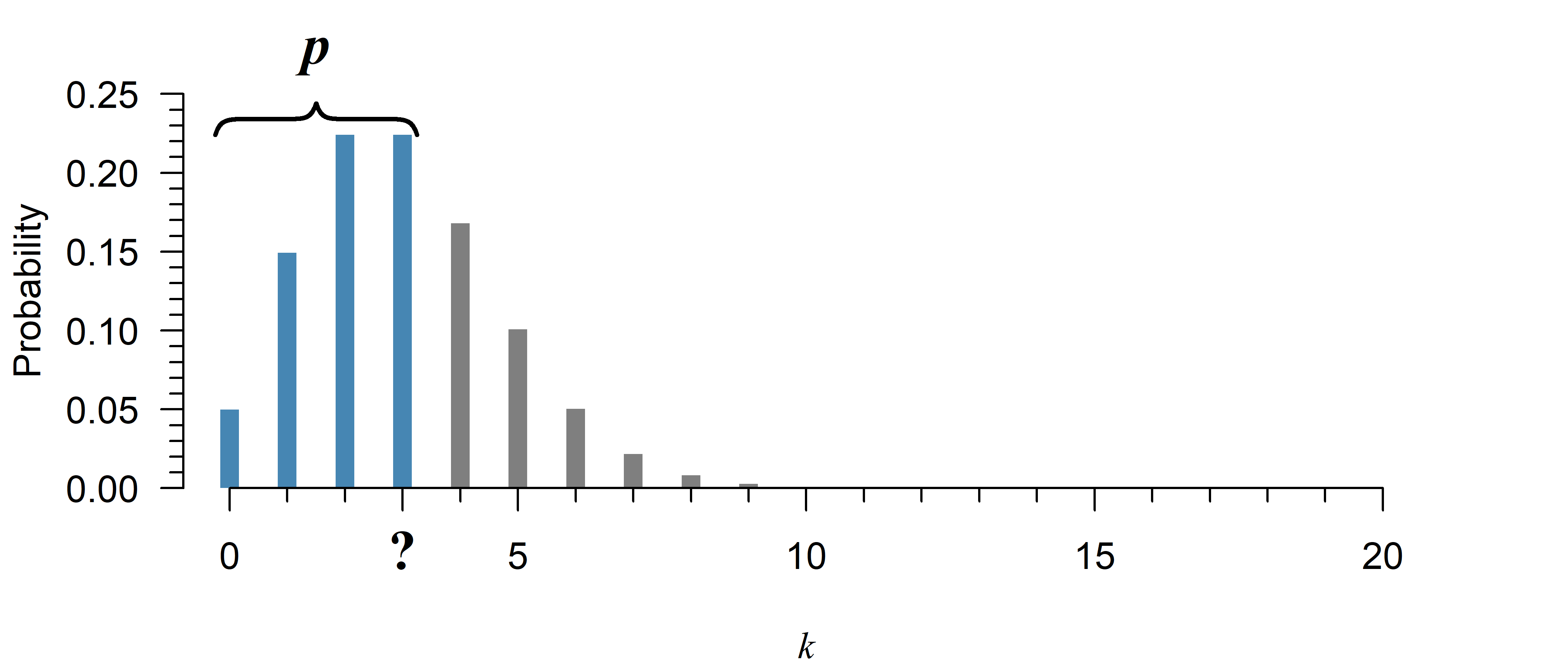
Suppose that in Figure 3, you need to know the value for \(k\) that has a total probability of at least 80%:

# The real answer:
qpois(0.8, lambda = 3)

[1] 4

# A numeric search using the CDF:
k <- 0
p <- ppois(k, lambda = 3)
while(p < 0.8){
  k <- k + 1
  p <- ppois(k, lambda = 3)
}
print(k)

[1] 4

The search stops at \(k=4\), because that is the first instance of a probability of at least 80%.

There are more efficient ways to go about this, but this is the underlying principle of R’s qpois and Python’s poisson.ppf.

Examples

R
Python

If there are on average 5 falling stars each night, what is the largest number of falling stars for 95% of all nights?

qpois(0.95, lambda = 5)

[1] 9

Within what range are the number of falling stars on 95% of all nights?

qpois(c(0.025, 0.975), lambda = 5)

[1]  1 10

Apparently, 95% of nights would have 1–10 falling stars if the average were 5.

If there are on average 5 falling stars each night, what is the largest number of falling stars for 95% of all nights?

from scipy.stats import poisson
poisson.ppf(0.95, 5)

9.0

Within what range are the number of falling stars on 95% of all nights?

result = poisson.ppf([0.025, 0.975], 5)
print(result)

[ 1. 10.]

Apparently, 95% of nights would have 1–10 falling stars if the average were 5.

Using the following code, you can plot the probability mass function of Poisson distribution with \(\lambda = 2\):

R
Python

x <- 0:20
y <- dpois(x, 2)
plot(y ~ x, type = "h", lwd = 4, lend = 1, las = 1)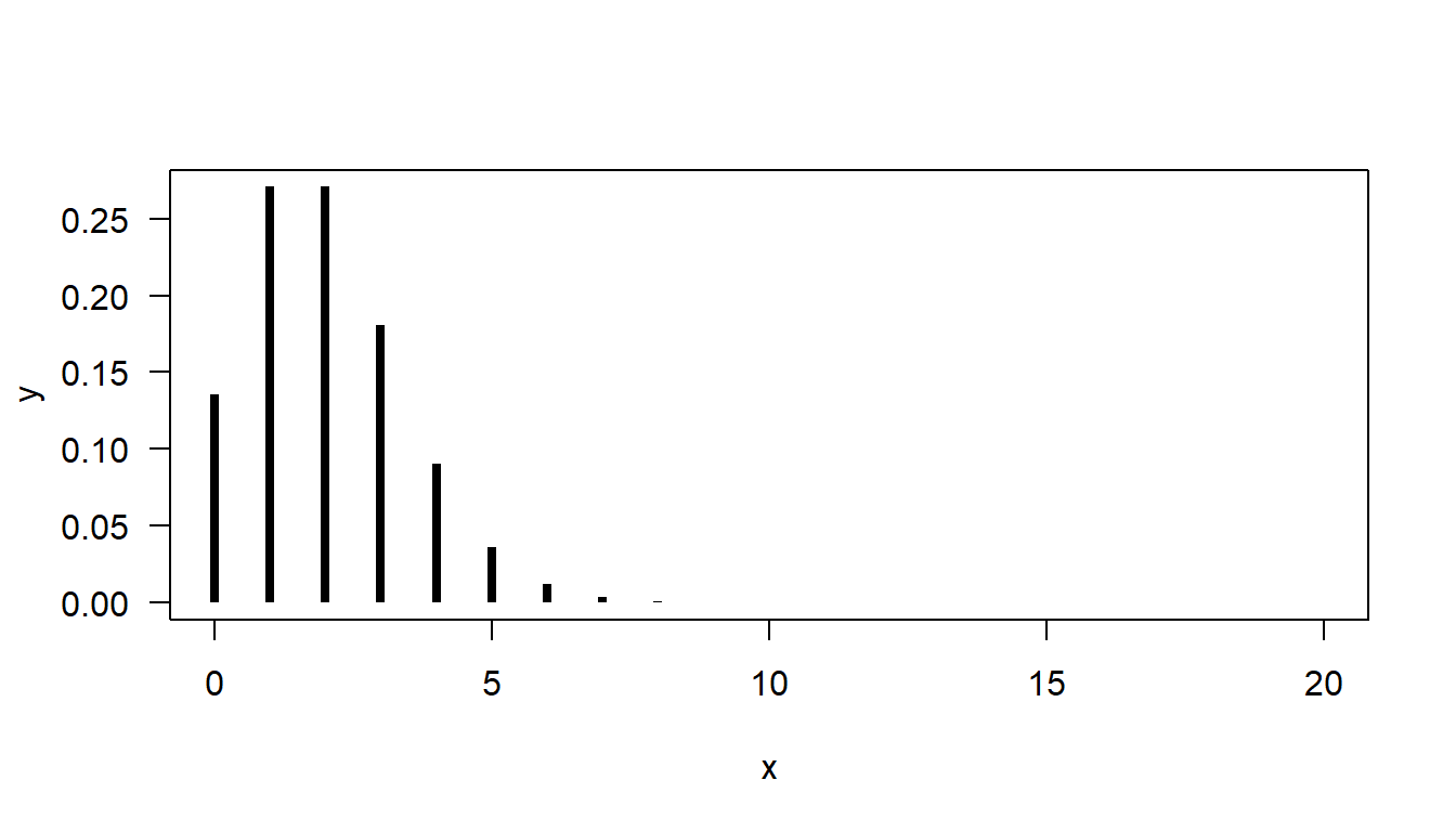

Try it in browser

(This is an experimental feature. I recommend just running RStudio in the background while reading this book, but perhaps this can be useful if you are reading this on your phone for example… Feedback is welcome!)

import numpy as np
from scipy.stats import poisson
import matplotlib.pyplot as plt

x = np.arange(0, 21)
y = poisson.pmf(x, 2)
plt.bar(x, y);
plt.show()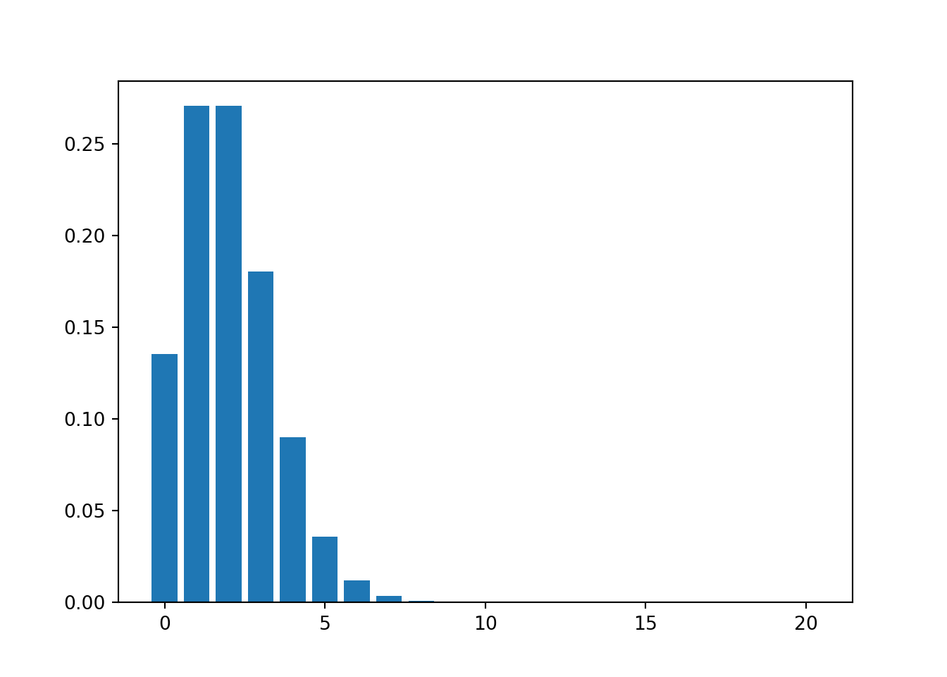

This probability distribution is:

Continuous / discrete
Left skewed / symmetric / right skewed

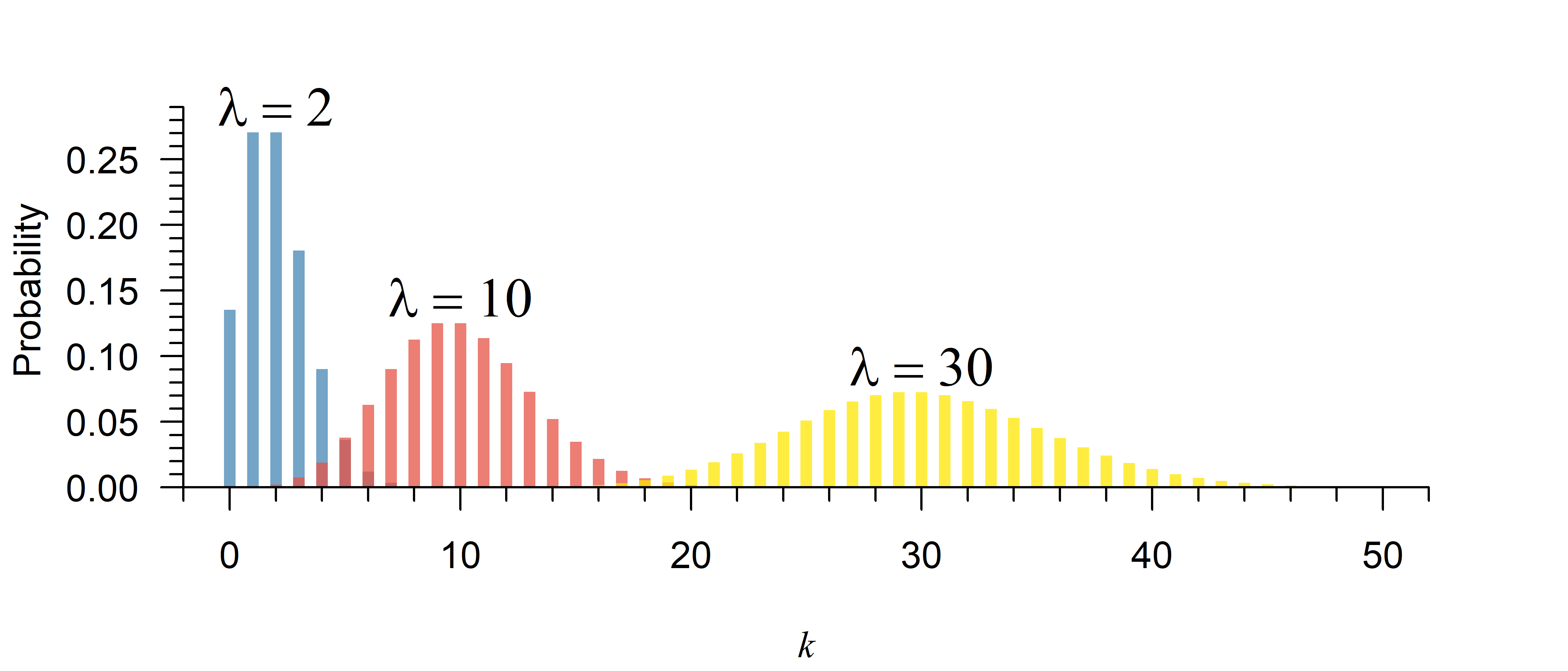
Try increasing the rate \(\lambda\) and plotting the result. The distribution is now:

More / less skewed

Do you understand why this is the case?

Hint

See the video on probability distributions (9:12).

A Poisson distribution with \(\lambda = 2\) is:

Continuous / discrete (Only certain values are possible)
Left skewed / symmetric / right skewed (The right tail is longer)

If you increase the rate \(\lambda\), the distribution is now:

More / less skewed (see Figure 4)

Explanation

Counts cannot be negative. If lambda is close to zero, the probability on the left side of the distribution gets pressed up into the side. If you increase lambda, you move further away from zero, so this skew becomes less apparent:

Figure 4: Increasing \(\lambda\) results in a more symmetric distribution.

Question 2
Answer

Perhaps the most commonly used laboratory animal is the mouse species C56BL/6. A study from 2015 estimated its litter size¹ to be approximately 7.5.[1]

Assuming litter size can be reasonably approximated with a Poisson distribution, what would be the chance of a litter size of at least 3?

C56BL/6 mouse. Source: jax.org/strain/003548

Hint

Use the code from exercise 1 to plot the distribution. This is the best way to get a feel for it.

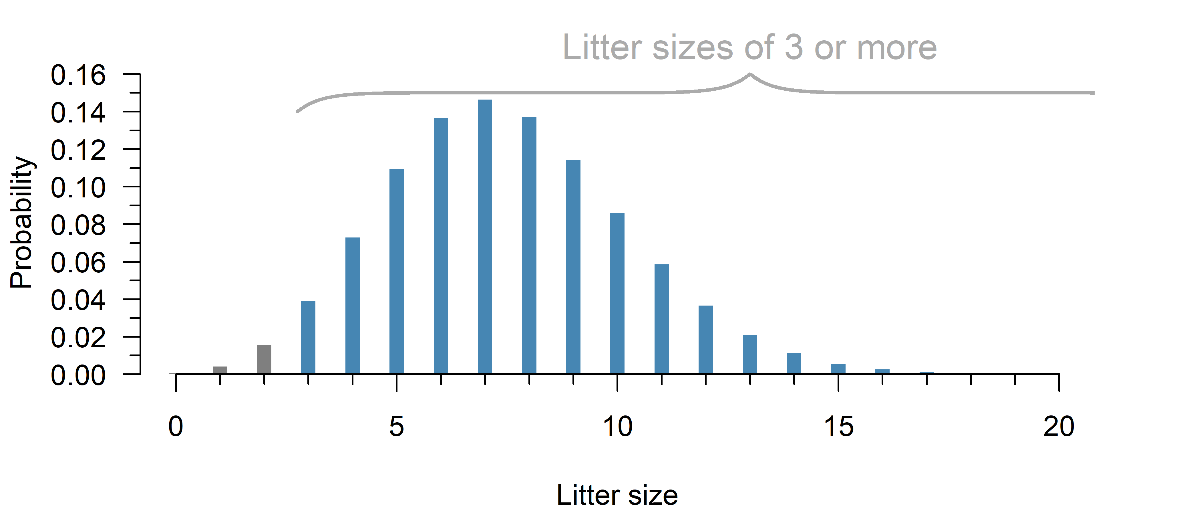
Now you can already see what would be a plausible answer: Almost all litter sizes are 3 or larger, so this should be well over 95%.

The question can be answered with the cumulative distribution function, see the explanation for details.

Try it in browser

Use the complement² of the cumulative distribution function:

R
Python

1 - ppois(2, 7.5)

[1] 0.9797433

from scipy.stats import poisson
1 - poisson.cdf(2, 7.5)

0.9797432849433356

If a Poisson distribution is a reasonable approximation, only about 2% of litters should be expected to have less than 3 mice.

Question 3
Answer

Continuing on question 2, within what values would you expect 80% of all litter sizes to be?

Hint

This can be answered with the quantile function.

Try it in browser

80% lies between the lowest 10% and highest 90%:

R
Python

qpois(c(0.1, 0.9), lambda = 7.5)

[1]  4 11

from scipy.stats import poisson
result = poisson.ppf([0.1, 0.9], 7.5)
print(result)

[ 4. 11.]

If a Poisson distribution is a reasonable approximation, the answer is 4–11 mice.

The number of offspring born at one time.↩︎
The cumulative distribution function gives you the left tail of the distribution. Hence, 1 minus the function gives you the right tail. This is called the complement.↩︎