2 Generalized Linear Models

Linear regression with counts, ratios, binary outcomes and more.

2.1 Lecture

Watch the videos on GLM and test your knowledge through the quiz questions. Then, apply your knowledge, by performing a complete analysis. The summary is meant as reference material to answer the quiz questions, should you get stuck.

Open playlist in a new tab

2.2 Summary

Figure 2.1: Example of a simple linear model. (Height and weight of 50 individuals.)

Mathematical formula:

As ordinary LM
As GLM

\[\begin{align} \label{lm} y &= \beta_0 + \beta_1 \cdot x + \epsilon \\ \tag{1a}\\ \epsilon &\sim \mathcal{N}(0, \, \sigma^2) \end{align}\]

\[\begin{align} \label{glmnorm} y|x &\sim \mathcal{N}(\mu, \, \sigma^2) \\ \\ \mu &= \eta\tag{1b}\\ \\ \eta &= \beta_0 + \beta_1 \cdot x \end{align}\]

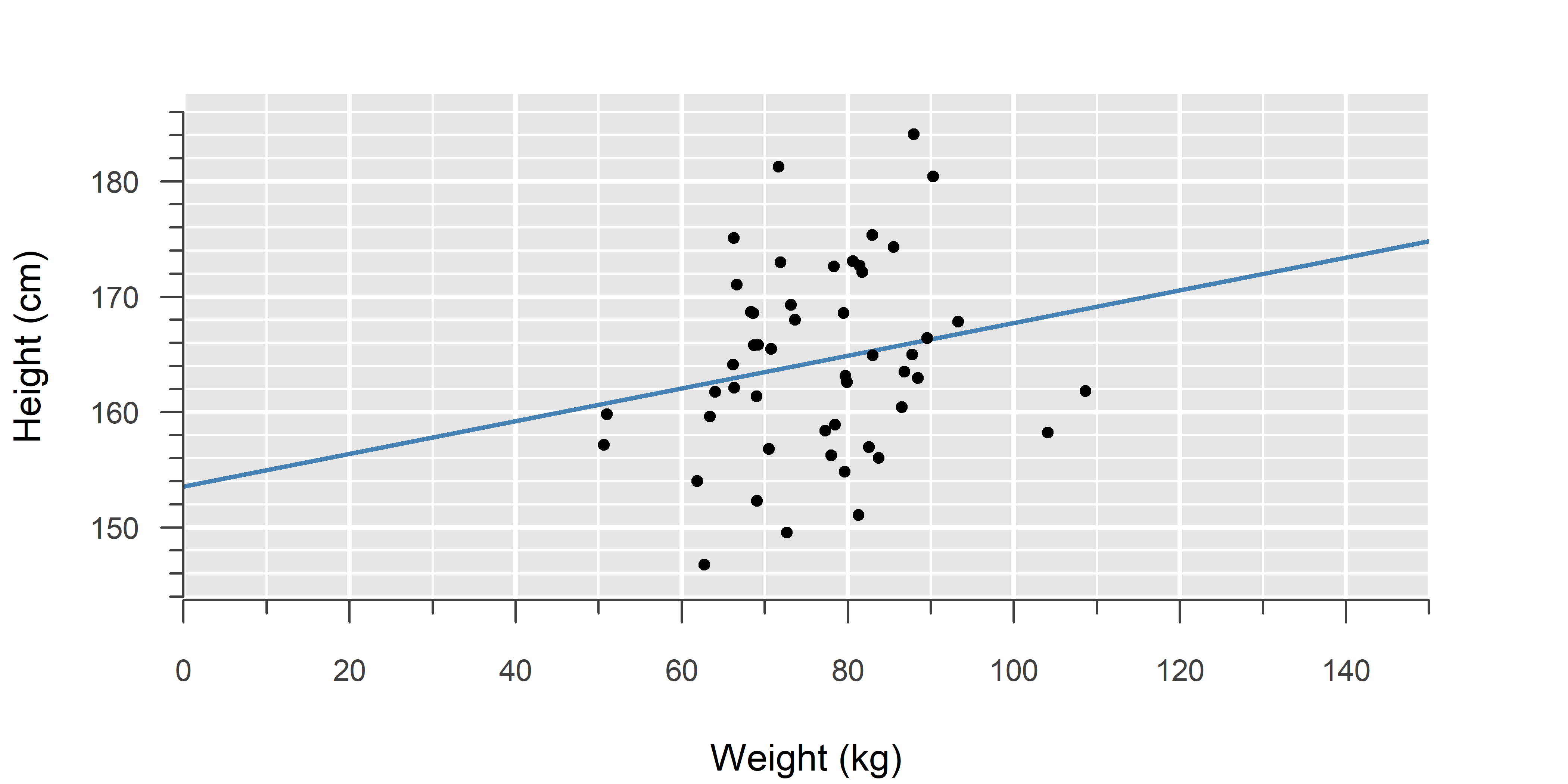
An ordinary linear model can also be written as a generalized linear model (GLM). This helps to see how ordinary linear models fit into the broader GLM framework.

Compare this to Poisson or binomial regression: In each case, we are estimating the mean of a distribution (here: $\mu$), and that mean changes depending on the explanatory variable ($x$).

The middle equation is the link function—how the mean relates to the linear equation ($\eta$). For a normal distribution, this is called the identity, which leaves the linear predictor unchanged, such that the linear equation is the mean of the resulting normal distribution.

Code:

R
Python

model <- lm(y ~ x, data)

import statsmodels.api as sm
model = sm.OLS(y, x).fit()

Note: You have to include an intercept manually using x = sm.add_constant(x).

Symbols & definitions

$y$ — response variable: The outcome.
$x$ — explanatory variable: The variable the outcome is regressed on.
$y|x$ — conditional response variable: The outcome at a given value of $x$.
$\mathcal{N}$ — normal distribution: See Normal Distribution. $y|x \sim \mathcal{N}\! \left(\mu, \, \sigma^2\right)$ means: The outcome follows a conditional normal distribution with mean $\mu$ and variance $\sigma^2$. It is called conditional, because $\mu$ is not a fixed number, but depends on $x$.
link function: A function that stretches the possible range of values of mean of the outcome to $-\infty$ to $+\infty$, which is convenient for estimating the model parameters, as it allows us to use a modified version of least squares (iteratively reweighted least squares).
canonical link function: The one link function that translates the linear predictor to the mean of the outcome. For the normal distribution, this is the identity function, which amounts to not doing any kind of transformation.
$\eta$ — linear predictor: The function that describes the relationship between the explanatory variable and the (transformed) mean of the outcome.
$\beta_0$ — intercept: Value of the outcome ($y$), when the explanatory variable ($x$) is zero. $\hat{\beta}_0$ (beta-hat) is its estimate.
$\beta_1$ — slope: Change in the outcome ($y$), when the explanatory variable ($x$) increases by one. $\hat{\beta}_1$ (beta-hat) is its estimate.

Explanation

Ordinary linear models are a special case of generalized linear models (GLMs). Whereas the former only support normally distributed errors, GLMs can handle any probability distribution in the exponential dispersion family.

To understand GLMs, try to let go of the idea that a linear model is $\text{linear function} + \text{error}$, and instead take on a different perspective: A GLM is a probability distribution with a mean that depends on the explanatory variable ($x$). The technical term for this is conditional normality: If we know the value of the $x$, then at that point, the outcome follows a normal distribution. Move to a different value of $x$ and the mean of the distribution changes. This concept is visualized in the first video on GLM.

Once we take on the perspective of a conditional probability distribution for the outcome, we can easily swap that distribution with another one, like Poisson or binomial. The only missing piece to do this is called the link function. Its purpose is to ensure the linear function will always output valid values (e.g., counts cannot be negative). If the link function also happens to coincide with the mean of the chosen probability distribution, it is called the canonical link function.

In the case of a normal distribution $\mathcal{N}\! \left(\mu, \, \sigma^2\right)$, the mean $\mu$ can already take on any value from $-\infty$ to $+\infty$, so no such translation is needed and we use what is called the identity function (it simply outputs the same value as the input). Since the identity link function coincides with the mean of the normal distribution, it is canonical.

When would you use a normal GLM with non-canonical link?

It is possible to use different link functions for a normal GLM (e.g., the logarithm). This is not the same as simply transforming the outcome. Below is an overview contrasting both methods.

Difference between log-transforming the outcome and using a log-link function.
	LM with $\log(y)$ as outcome	Normal GLM with log-link
Rationale	You expect the outcome (including the errors) to grow exponentially with the explanatory variable. Errors grow larger as $y$ increases.	You expect the trend (excluding errors) to be exponential. Error variance is constant along this trend.
Example	Someone who spends $100 on average will have smaller absolute spread in spending than someone who spends $1,000 on average.	A deterministic process like laser intensity as a function of distance still has measurement error. This can cause a constant spread along an exponential relationship.
Disadvantage	Transforming back to the original scale is not straightforward, due to retransformation bias and requires e.g., a smearing estimate [1].	Less common in practice. In most real-world processes, if something grows exponentially, its spread tends to grow exponentially too.

Example

Refer to the previous chapter.

Mathematical formula:

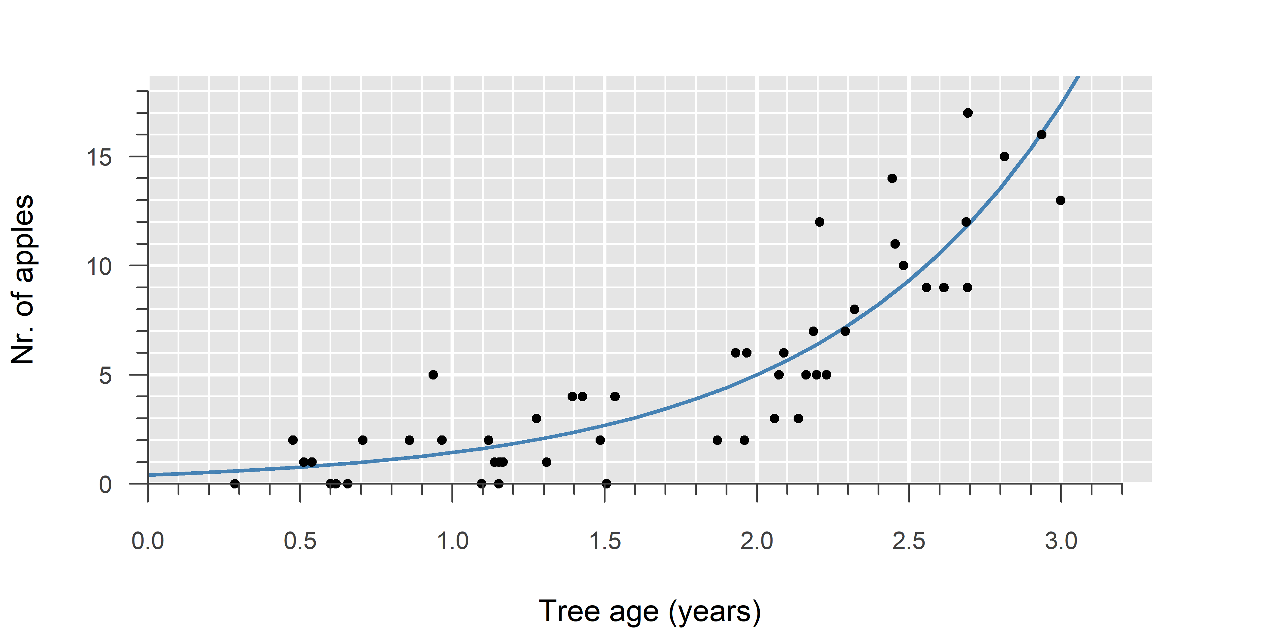
\[\begin{align} \label{glmpois} y|x &\sim \mathsf{Pois}(\lambda) \\ \\ \tag{2}\log(\lambda) &= \eta \\ \\ \eta &= \beta_0 + \beta_1 \cdot x \end{align}\]

Code:

R
Python

model <- glm(y ~ x, data, family = "poisson")

import statsmodels.api as sm
model = sm.GLM(y, X, family = sm.families.Poisson()).fit()

Note: You have to include an intercept manually using X = sm.add_constant(X).

Symbols & definitions

$y$ — response variable: The outcome.
$x$ — explanatory variable: The variable the outcome is regressed on.
$y|x$ — conditional response variable: The outcome at a given value of $x$.
$\mathsf{Pois}$ — Poisson distribution: See Poisson Distribution. $y|x \sim \mathsf{Pois}(\lambda)$ means: The outcome follows a conditional Poisson distribution with rate $\lambda$. It is called conditional, because $\lambda$ is not a fixed number, but depends on $x$.
link function: A function that stretches the possible range of values of mean of the outcome to $-\infty$ to $+\infty$, which is convenient for estimating the model parameters, as it allows us to use a modified version of least squares (iteratively reweighted least squares).
canonical link function: The one link function that translates the linear predictor to the mean of the outcome. For the Poisson distribution, this is the natural logarithm: $\log(\lambda)$
$\eta$ — linear predictor: The function that describes the relationship between the explanatory variable and the (transformed) mean of the outcome.
$x$ — explanatory variable: The variable the outcome is regressed on.
$\beta_0$ — intercept: Value of the outcome ($y$), when the explanatory variable ($x$) is zero. $\hat{\beta}_0$ (beta-hat) is its estimate.
$\beta_1$ — slope: Change in the outcome ($y$), when the explanatory variable ($x$) increases by one. $\hat{\beta}_1$ (beta-hat) is its estimate.

Explanation

A Poisson GLM is used to model count data. It is the model of choice when counts are truly independent and occur at a fixed rate—that is, when the rate depends only on the explanatory variable ($x$).

In a Poisson GLM, we estimate the rate of occurrence ($\lambda$). Since events cannot occur at a negative rate, a suitable link function must ensure $\lambda \geq 0$. A common choice is the natural logarithm $\log(\lambda) = \eta$, because it implies $\lambda = e^{\eta}$ (always positive). This is also the canonical link function of a Poisson GLM. An example of a non-canonical link function is the square root $\sqrt{\lambda} = \eta$.

In practice, counts are often correlated, zero-inflated, or otherwise not truly independent and occurring at a fixed rate. For an explanation of this topic, as well as alternatives to Poisson regression, refer to the fourth video on GLM.

Example

Refer to the tutorials below.

Example: Ratio
Example: Binary

Figure 2.3: Example of logistic regression. (Correct questions as a function of studying time.)

Mathematical formula:

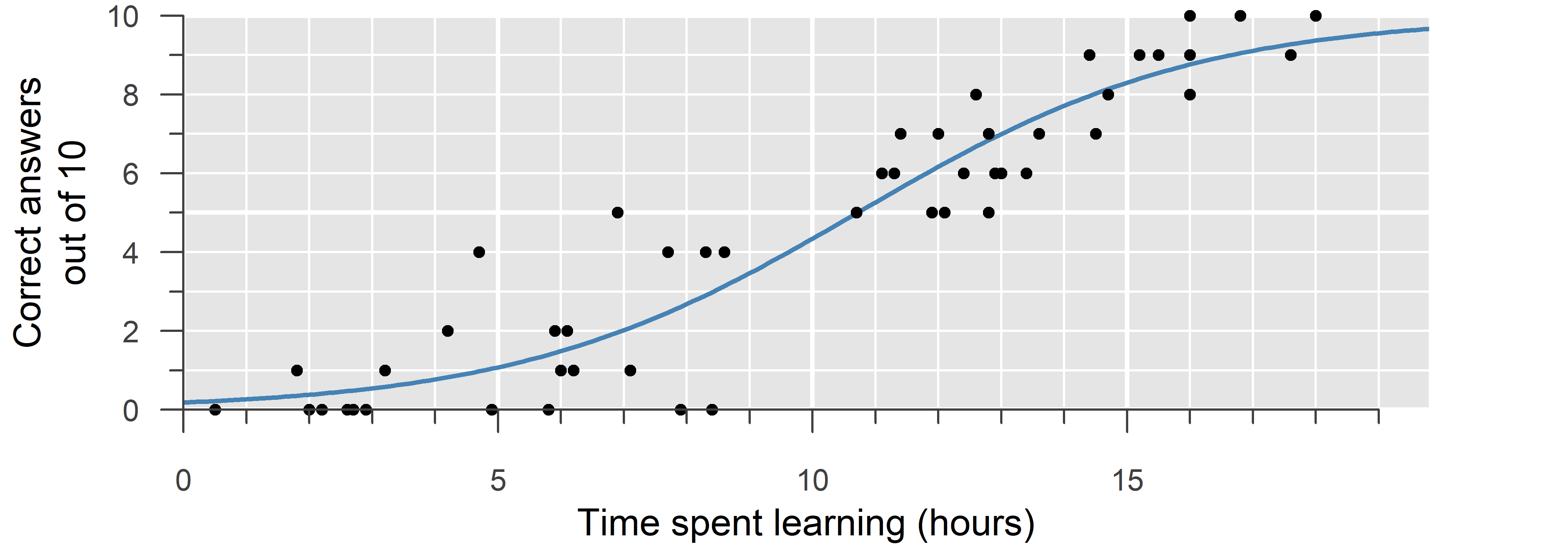
\[\begin{align} \label{glmbinom} y|x &\sim \mathsf{Binom}(n, \, p) \\ \\ \tag{3a}\log \left( \frac{p}{1-p} \right) &= \eta \\ \\ \eta &= \beta_0 + \beta_1 \cdot x \end{align}\]

Code:

R
Python

model <- glm(cbind(success, failure) ~ x, data, family = "binomial")

import statsmodels.api as sm
model = sm.GLM(y, X, family = sm.families.Binomial()).fit()

Note: You have to include an intercept manually using X = sm.add_constant(X).

Figure 2.4: Example of logistic regression. (Probability of passing as a function of studying.)

Mathematical formula:

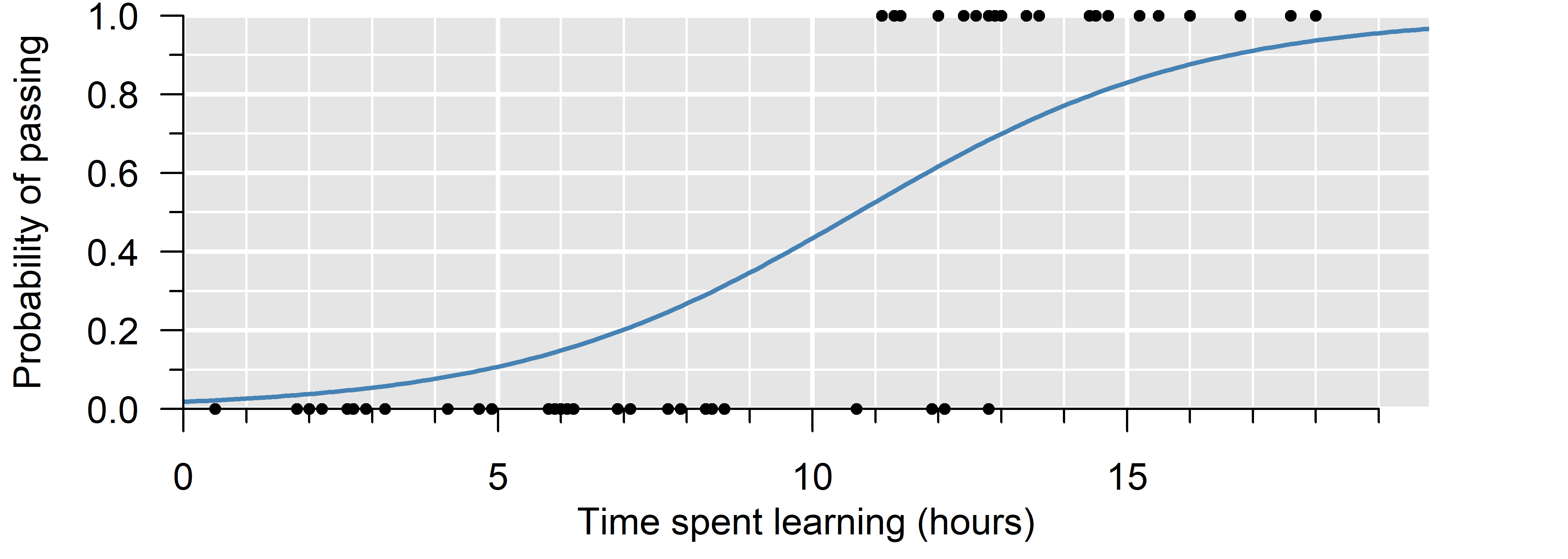
\[\begin{align} \label{glmbern} y|x &\sim \mathsf{Bernoulli}(p) \\ \\ \tag{3b}\log \left( \frac{p}{1-p} \right) &= \eta \\ \\ \eta &= \beta_0 + \beta_1 \cdot x \end{align}\]

Code:

R
Python

model <- glm(y ~ x, data, family = "binomial")

import statsmodels.api as sm
model = sm.GLM(y, X, family = sm.families.Binomial()).fit()

Note: You have to include an intercept manually using X = sm.add_constant(X).

Symbols & definitions

$y$ — response variable: The outcome.
$x$ — explanatory variable: The variable the outcome is regressed on.
$y|x$ — conditional response variable: The outcome at a given value of $x$.
$\mathsf{Binom}$ — binomial distribution: See Binomial Distribution. $y|x \sim \mathsf{Binom}(n, \, p)$ means: The outcome follows a conditional binomial distribution with $n$ trials and probability of success $p$. It is called conditional, because $p$ is not a fixed number, but depends on $x$.
$\mathsf{Bernoulli}$ — Bernoulli distribution: A binomial distribution with one trial simplifies to what is called the Bernoulli distribution.
link function: A function that stretches the possible range of values of mean of the outcome to $-\infty$ to $+\infty$, which is convenient for estimating the model parameters, as it allows us to use a modified version of least squares (iteratively reweighted least squares).
canonical link function: The one link function that translates the linear predictor to the mean of the outcome. For the binomial distribution, this is the logarithm of the odds, or logit: $\log \left( \frac{p}{1-p} \right)$
$\eta$ — linear predictor: The function that describes the relationship between the explanatory variable and the (transformed) mean of the outcome.
$x$ — explanatory variable: The variable the outcome is regressed on.
$\beta_0$ — intercept: Value of the outcome ($y$), when the explanatory variable ($x$) is zero. $\hat{\beta}_0$ (beta-hat) is its estimate.
$\beta_1$ — slope: Change in the outcome ($y$), when the explanatory variable ($x$) increases by one. $\hat{\beta}_1$ (beta-hat) is its estimate.

Explanation

A binomial GLM is used to model ratios and binary outcomes. It is the model of choice when the trials are truly independent and the probability of success fixed—that is, when the probability of success depends only on the explanatory variable ($x$).

In a binomial GLM, we estimate the probability of success ($p$). Since probabilities must be within $0$ and $1$, a suitable link function must ensure $0 \leq p \leq 1$. A common choice is the logit \[\log\left(\frac{p}{1 - p}\right) = \eta \quad \implies \quad p = \frac{1}{1 + e^{-\eta}}\] which is between $0$ and $1$ for any value of $\eta$. This is also the canonical link function of a binomial GLM. Examples of non-canonical link functions include the probit $\Phi^{-1}(p) = \eta$ and the complementary log-log $\log(-\log(1 - p)) = \eta$.

Often, trials are correlated or otherwise not truly independent and occurring with a fixed probability of success. For an explanation of this topic, as well as alternatives to binomial regression, refer to the fourth video on GLM.

Finally, if you have the choice—such as during the study design phase—always use the original number of successes and failures, not a percentage or proportion. Computing a percentage discards valuable information (i.e., the number of trials).

Example

Refer to the tutorials.

Which of the following is implicitly assumed in a generalized linear model? (choose one)

A. The data follow a distribution in the exponential dispersion family
B. The outcome follows a distribution in the exponential dispersion family
C. The residuals follow a distribution in the exponential dispersion family
D. The outcome conditionally follows a distribution in the exponential dispersion family

Hint

See the first video on GLM.

Which of the following is implicitly assumed in a generalized linear model? (choose one)

A. The data follow a distribution in the exponential dispersion family
B. The outcome follows a distribution in the exponential dispersion family
C. The residuals follow a distribution in the exponential dispersion family
D. The outcome conditionally follows a distribution in the exponential dispersion family

Learn why

The distributional assumption is about the conditional outcome, which means: At any given value of the explanatory variable ($x$), the outcome is assumed to follow the specified distribution. But the unconditional outcome (disregarding the value of $x$) is not assumed to follow anything.

In mathematical terms,

\[\begin{aligned} y &\not\sim \text{probability distribution} \\ \\ y|x &\sim \text{probability distribution} \end{aligned}\]

GLMs make no assumptions about your entire data set, nor your outcome variable. The residuals are also irrelevant, as a GLM has no error term in its equation. The randomness instead comes from the specified probability distribution.

Question 2
Answer

Which probability distributions are associated with these processes?

The number of bees visiting flowers in one minute.
The number of germinated seeds in a pot, out of 20 planted.
Cortisol concentration in blood plasma samples (ng/mL).
Presence or absence of sharks in different locations.

Hint

Choose from among: normal, Poisson, Bernoulli, binomial.

Which probability distributions are associated with these processes?

The number of bees visiting flowers in one minute. Poisson
The number of germinated seeds in a pot, out of 20 planted. binomial
Cortisol concentration in blood plasma samples (ng/mL). normal
Presence or absence of sharks in different locations. Bernoulli

Learn why

The number of bees per minute is a count over a fixed time window, so a starting point would be a Poisson distribution.
The number of germinated seeds sounds like a count, but beware: there is a hard upper limit ($20$ seeds planted). Hence, it is better to consider this the number of successes out of $20$ trials (a ratio), which can be modeled with a binomial distribution.
Concentration is a continuous outcome, so a starting point could be an ordinary linear model (normal distribution). If cortisol concentrations turn out to be highly skewed, we could try transformation (e.g., modeling $\log_{10}(\mathrm{concentration})$ instead), or using a distribution that can be right-skewed, like the gamma distribution.
If we don’t count sharks, but simply note their presence/absence, this is a binary outcome. This can be modeled with a binomial distribution with a single trial. This is also called a Bernoulli distribution.

Question 3
Answer

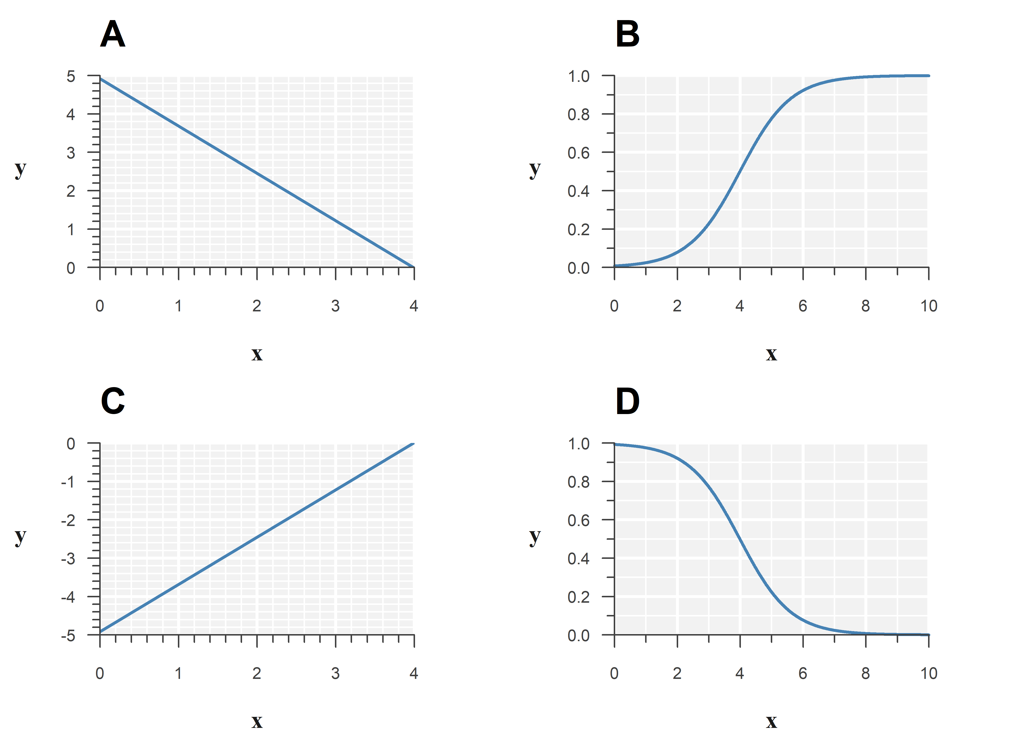
Below is the output of a binomial GLM with logit link function:

             Estimate Std. Error   z value     Pr(>|z|)
(Intercept)  4.918964  0.2945861 16.697883 1.357977e-62
x           -1.233567  0.2264006 -5.448604 5.076661e-08

Which of the following best represents the model?

Hint

Consider the effect the link function has on the estimated relationship.

Below is the output of a binomial GLM with logit link function:

             Estimate Std. Error   z value     Pr(>|z|)
(Intercept)  4.918964  0.2945861 16.697883 1.357977e-62
x           -1.233567  0.2264006 -5.448604 5.076661e-08

Option D best represents the model:

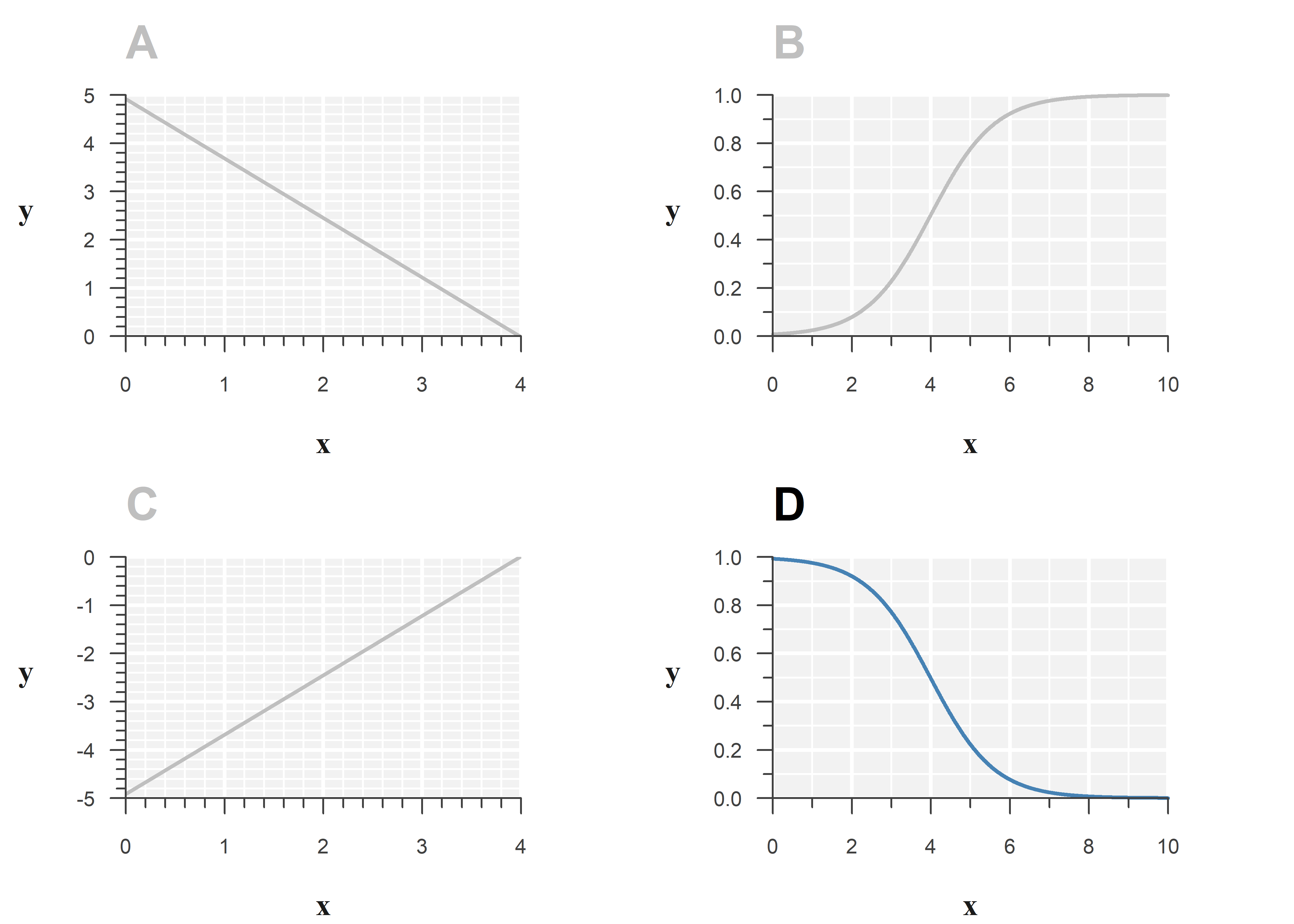
Learn why

Filling in the estimates, the fitted model is:

\[\begin{align} \log \left( \frac{p}{1-p} \right) &= \eta \\ \\ \hat{\eta} &= \texttt{4.919} - \texttt{1.234} \cdot x \end{align}\]

The estimated slope is negative, so the S-shape should go down when $x$ increases.

While you cannot quickly evaluate $\mathrm{logit}(\eta)$ by hand, this question can be answered by elimination: A and C cannot be correct, as the logit link function does not result in a straight line. B is also incorrect as the estimated slope of $x$ is negative.

Question 4
Answer

Which statements are correct?

Overdispersion leads to poor estimates of the intercept and slope.
Correlation among observations can cause both over- and underdispersion.
Overdispersion can be resolved by changing link functions.
Counts are always (conditionally) Poisson distributed.
A negative binomial distribution can be used to model count data.
Ordinary linear models cannot be overdispersed.

Hint

All of these are covered in the fourth video on GLM.

Which statements are correct?

Overdispersion leads to poor estimates of the intercept and slope.
Correlation among observations can cause both over- and underdispersion.
Overdispersion can be resolved by changing link functions.
Counts are always (conditionally) Poisson distributed.
A negative binomial distribution can be used to model count data.
Ordinary linear models cannot be overdispersed.

Learn why

Overdispersion means that at any predicted value of the outcome, there is more spread in observed values than you would expect. This means 1 is incorrect, because the issue is not the estimates but their uncertainty (standard errors).
Positive correlation leads to overdispersion, whereas negative correlation leads to underdispersion, as shown in the video on overdispersion . Hence, 2 is correct.
Changing a link function changes the estimated relationship (although usually the effect is small). For the same reason as 1 then, 3 is incorrect, as excess spread is not addressed this way.
A Poisson distribution does arise in theory if counts are independent and occurring at a fixed rate. However, in real life, these are rarely realistic assumptions and at best, they hold approximately. Hence, 4 is incorrect.
Despite the name, negative binomial is an alternative to the Poisson (not binomial) distribution that is commonly used to address overdispersion. Hence, 5 is correct.
Overdispersion happens because the Poisson and binomial distribution only have a single free parameter ($\lambda$ and $p$, respectively). In ordinary linear models, there is a separate parameter for the variance ($\sigma^2$), so it is not possible to have overdispersion. Hence, 6 is correct. Variance is not always constant in ordinary linear models, but that is a separate issue.

Question 5
Answer

An ordinary linear model (LM) is a special case of a generalized linear model (GLM). Can you verify this from the output?

R
Python

Run the code below and compare the output of lm with that of glm.

# Ordinary linear model
LM <- lm(Sepal.Length ~ Petal.Length, data = iris)
summary(LM)

# Generalized linear model
GLM <- glm(Sepal.Length ~ Petal.Length, data = iris, family = "gaussian")
summary(GLM)

Try it in browser

Run the code below and compare the output of sm.OLS with that of sm.GLM.

import pandas as pd
import statsmodels.api as sm

# Ordinary linear model
iris = sm.datasets.get_rdataset('iris').data
X = iris['Petal.Length']
y = iris['Sepal.Length']
X = sm.add_constant(X) # Add an intercept
model = sm.OLS(y, X).fit()
print(model.summary2())

# Generalized linear model
iris = sm.datasets.get_rdataset('iris').data
X = iris['Petal.Length']
y = iris['Sepal.Length']
X = sm.add_constant(X) # Add an intercept
model = sm.GLM(y, X, family = sm.families.Gaussian()).fit()
print(model.summary2())

An ordinary linear model (LM) is a special case of a generalized linear model (GLM). Can you verify this from the output?

R
Python

Run the code below and compare the output of lm with that of glm.

# Ordinary linear model
LM <- lm(Sepal.Length ~ Petal.Length, data = iris)
summary(LM)

# Generalized linear model
GLM <- glm(Sepal.Length ~ Petal.Length, data = iris, family = "gaussian")
summary(GLM)

Both methods produce identical estimates and standard errors, demonstrating that a normal GLM is not fundamentally different than an ordinary linear model.

Learn why

Focusing on the coefficients first, we can quickly verify that the estimates and their standard errors are indeed identical:

summary(LM)$coefficients

              Estimate Std. Error  t value      Pr(>|t|)
(Intercept)  4.3066034 0.07838896 54.93890 2.426713e-100
Petal.Length 0.4089223 0.01889134 21.64602  1.038667e-47

summary(GLM)$coefficients

              Estimate Std. Error  t value      Pr(>|t|)
(Intercept)  4.3066034 0.07838896 54.93890 2.426713e-100
Petal.Length 0.4089223 0.01889134 21.64602  1.038667e-47

Differences between lm and glm include:

lm shows a simple summary of the residuals, glm does not. This is because GLMs are not limited to normally distributed errors, so it does not necessarily help to inspect the residuals. (For distributions other than normal, there is no possible decomposition in to $\text{linear function} + \text{error}$.)
lm shows a $t$-value, but glm a $z$-value for the estimates. The reasons for this is a bit technical, but it boils down to the lack of an error term in a GLM. A longer explanation is included at the end.
lm shows $R^2$ and $R^2_{\mathrm{adjusted}}$, a GLM does not. This is because GLMs do not explain variance ($\sigma^2$), but a more broad definition of spread, called deviance.
glm does not show the residual standard deviation for the same reason.
lm includes an omnibus $F$-test. This test is not suitable for GLMs, so it is not included in the output of glm.
glm shows the null and residual deviance. Deviance is a measure of spread that applies more generally than the variance ($\sigma^2$).
- This gives you a similar piece of information as $R^2$ does in lm: There was originally a deviance of 102.168, and only 24.525 left.
- In the special case of a normal GLM, the deviance explained coincides with the variance explained: $1 - \frac{\texttt{24.525}}{102.168} = 76\%$, again showing that an ordinary linear model is the same as a normal GLM with identity link.
glm shows the Akaike information criterion (AIC) value by default, lm does not. This difference is superficial, as AIC is well-defined for both models (try AIC(LM)). Note that this number is useless in isolation—it is only useful when comparing models.
At the bottom, glm shows the number of iterations it took for the fitting procedure to converge, by means of Fisher scoring. This is a fast method for obtaining the estimates of a GLM, which is not used in lm.

Technical explanation: $t$-values vs $z$-values

A $t$-value follows a $t$-distribution, a $z$-value a normal distribution.

In an ordinary linear model, we make assumptions about the error ($\epsilon$). If the error is truly normally distributed, then the residual (the ‘estimate’ of the error) follows an exact, known distribution, namely, a $t$-distribution with degrees of freedom equal to the residual degrees of freedom.

By contrast, a GLM cannot be decomposed into $\text{linear function} + \text{error}$. Instead, the assumptions are made about the conditional distribution of the outcome ($y$). Hence, the $p$-values shown in the regression table of a GLM are based on something else entirely: Asymptotically (if $n \to \infty$), the distribution of the maximum likelihood estimator of $\beta$ tends to a normal distribution, irrespective of the type of GLM distribution family, and so a $z$-value is asymptotically justified, as long as the model assumptions hold.

In practice, model assumptions rarely hold exactly. Hence, this technical difference is not so important, and there also exist better, more general methods of obtaining $p$-values and confidence intervals, like bootstrapping.

Run the code below and compare the output of sm.OLS with that of sm.GLM.

import pandas as pd
import statsmodels.api as sm

# Ordinary linear model
iris = sm.datasets.get_rdataset('iris').data
X = iris['Petal.Length']
y = iris['Sepal.Length']
X = sm.add_constant(X) # Add an intercept
model = sm.OLS(y, X).fit()
print(model.summary2())

# Generalized linear model
iris = sm.datasets.get_rdataset('iris').data
X = iris['Petal.Length']
y = iris['Sepal.Length']
X = sm.add_constant(X) # Add an intercept
model = sm.GLM(y, X, family = sm.families.Gaussian()).fit()
print(model.summary2())

Both methods produce identical estimates and standard errors, demonstrating that a normal GLM is not fundamentally different than an ordinary linear model.

Learn why

…

2.4 Apply your knowledge

Below you can find a worked out example (tutorial) and a dataset for you to analyze yourself (exercise):

Tutorial — Poisson (qmd , data )
Tutorial — binomial (qmd , data )
Exercise (qmd , data )

How to read data in R

Save the data and qmd file in the same location on your computer.
Open the qmd file in RStudio.
Set working directory to source file location.
(Session > Set Working Directory > To Source File Location)
R will now read from the folder the qmd file is located, so you can just use read.csv("name-of-data.csv").