Chapter 3 Mendelian Genetics
Date: 21/22 September 2021
Topic: Probability theory, hypothesis testing
Duration: 30–90 min.
In this chapter you will learn how to compare observed to expected frequencies using a chi-squared test.
3.1 Corn Example
In the basic practicals you will count the number of differently colored corn kernels.
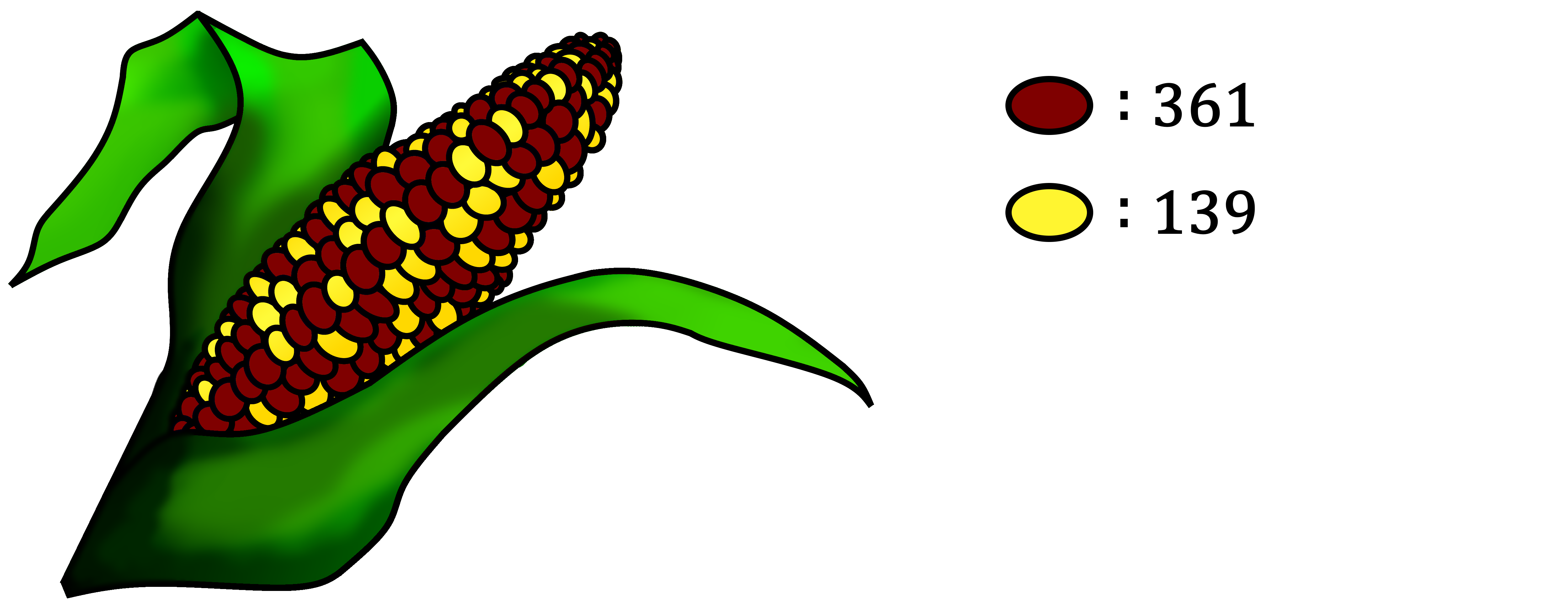
Figure 3.1: A cob of corn with differently colored kernels.
According to Mendelian genetics, if both parents were heterozygous for one color-causing gene, then we would expect a \(3 : 1\) ratio of kernels with dominant to recessive trait. For example, consider heterozygous parents for the red color-causing gene R:
| R | r | |
|---|---|---|
| R | RR (red) | Rr (red) |
| r | Rr (red) | rr (yellow) |
If both parents were indeed Rr, then we would expected \(\text{red} : \text{yellow} = 3 : 1\) in the offspring.
A statistical test works by taking on a statement of no difference and then collecting evidence against it. For the chi-squared test, that means that we compare the observed frequencies to the frequencies we would get under a \(3:1\) ratio. You can calculate these expected frequencies simply by multiplying the total kernels counted with the expected proportion. (Take care to convert the ratio to a proportion first.)
Exercise 1
Suppose you count \(361\) red kernels and \(139\) yellow ones. What are the expected number of red and yellow kernels under the null-hypothesis of a \(3 : 1\) ratio?
Exercise 2
The chi-squared test is defined as follows:
\[\begin{equation} \displaystyle\chi^2 = \sum_{i = 1}^k \frac{(\text{observed}_i - \text{expected}_i)^2}{\text{expected}_i} \tag{3.1} \end{equation}\]
Where \(k\) is the number of groups. Since there are only two groups (red, yellow), this becomes:
\(\displaystyle\chi^2 = \frac{(\text{observed}_\text{red} - \text{expected}_\text{red})^2}{\text{expected}_\text{red}} + \frac{(\text{observed}_\text{yellow} - \text{expected}_\text{yellow})^2}{\text{expected}_\text{yellow}}\)
Calculate \(\chi^2\) using the observed and expected numbers from exercise 1. Show your calculation.
3.2 Chi-Squared Test
In R you can compare observed to expected frequencies using chisq.test:
example <- c(361, 139)
chisq.test(example, p = c(3/4, 1/4)) # Test against a 3:1 ratio
##
## Chi-squared test for given probabilities
##
## data: example
## X-squared = 2.0907, df = 1, p-value = 0.1482This test calculates \(\chi^2\) and computes a corresponding \(p\)-value that has the following meaning:
- If the population has a \(3 : 1\) ratio of red to yellow kernels, what is the chance of observing at least this large a deviation?1
If this chance is very small, then perhaps the null-hypothesis of a \(3 : 1\) ratio is not realistic and we reject it. If it is large, then this corn cob might as well have arisen from parents that yield a \(3 : 1\) ratio, and we don’t reject the null-hypothesis.
So what is small and large? That is a matter of opinion, but in biology a value of \(0.05\) is often used as a boundary. That means there is a \(\frac{1}{20}\) chance of incorrectly concluding a significant deviation from \(3 : 1\).
Exercise 3
Look at the output from the chi-squared test. With a threshold of \(0.05\), would you reject the null-hypothesis? What do you conclude?
Exercise 4
Perform the same \(\chi^2\)-test for your own counts of a corn cob and report the conclusion. Use the code from the example and adapt it for your own counts.
Exercise 5 (optional)
In the basic practicals, it was explained that all of four different dominant mutations are required for there to be red kernels: C, R, A1 and A2.
Since these are all dominant mutations, let’s assume that each mutant protein has a \(\frac{3}{4}\) chance of being present in the offspring (due to a \(3 : 1\) ratio). What is then the chance of a red kernel?
(For simplicity, ignore the possibility of C-inhibitor.)
Population here does not refer to a biological population, but a statistical population. It is the population of all possible red and yellow corn kernels that could have formed from a \(3 : 1\) ratio.↩︎