Tutorial 10 Reading & Storing Data
This chapter provides some advice for how to store data and shows you various ways in which you can read it.
Summary
- Store data in tidy format. There are exceptions to this format, but only one for the methods listed on this website; (namely, long-format for time series)
- Separate data entry and analysis. Excel invites you to do questionable things, like adding figures and explanation to raw data. Don’t do this. Never edit or clutter raw data. If you must use Excel for data exploration, create a separate file for this purpose.
- Use short, informative variable names, using only lower- and uppercase letters, numbers,1 and if needed periods (.) or underscores (_). Do not add the unit of measurement, or any explanation. This belongs in the meta data. If variable names are still long, consider using abbreviations. Avoid special characters (!@#$%^&*-a=+,<>?/).
- Keep a meta data file, or sheet, that explains variables, abbreviations, unit of measurement, etc. See here for an example. This also helps keep variable names short and free of special characters.
- Save data as comma-separated values (.csv), rather than as an Excel file (.xlsx). Saving into this format automatically removes any content statistical software cannot read anyway, like figures and coloring. This file format is suitable for most sizes of data commonly encountered in the life sciences (anything that still fits into RAM on an ordinary computer).
10.1 Tidy Format
Collect data in a simple, consistent format called tidy data,9 such that minimal effort is required to clean the data once you get to the analysis: Rows represent observations, columns represent the variables measured for those observations:
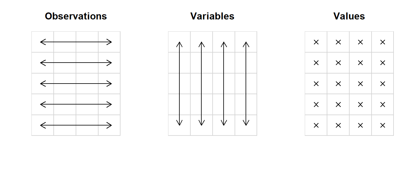
Figure 10.1: The basic principle of tidy data. This data set has 5 observations of 4 variables.
Good example
The iris data set (preinstalled with R) is in tidy format:
| Sepal.Length | Sepal.Width | Petal.Length | Petal.Width | Species |
|---|---|---|---|---|
| 5.1 | 3.5 | 1.4 | 0.2 | setosa |
| 4.9 | 3.0 | 1.4 | 0.2 | setosa |
| 4.7 | 3.2 | 1.3 | 0.2 | setosa |
| 4.6 | 3.1 | 1.5 | 0.2 | setosa |
| 5.0 | 3.6 | 1.4 | 0.2 | setosa |
| … | … | … | … | … |
Here, the rows each represent one observation (a distinct flower), and the columns represent the variables measured/recorded (physical dimensions and species).
Bad example
A common deviation from tidy format is to represent groups as columns:
| women | men |
|---|---|
| 114 | 123 |
| 121 | 117 |
| 125 | 117 |
| 108 | 117 |
| 122 | 116 |
Do you have different groups? Time points? Replicates of the experiment? Then try to adhere to the same principle: Columns are variables. Simply add a variable that indicates which group/time point/replicate this observation belongs to:
| sex | SBP |
|---|---|
| female | 114 |
| female | 121 |
| female | 125 |
| female | 108 |
| female | 122 |
| male | 123 |
| male | 117 |
| male | 117 |
| male | 117 |
| male | 116 |
Converting to tidy format
If you have data split by group/time point/replicate here is how you can convert it to tidy format:
# The untidy data set
Untidy
## women men
## 1 114 123
## 2 121 117
## 3 125 117
## 4 108 117
## 5 122 116# Convert by hand
Tidy <- data.frame(
sex = rep(c("female", "male"), each = nrow(Untidy)),
SBP = c(Untidy$women, Untidy$men)
)
# Convert using a package (install if missing)
library("reshape2")
melt(Untidy)## variable value
## 1 women 114
## 2 women 121
## 3 women 125
## 4 women 108
## 5 women 122
## 6 men 123
## 7 men 117
## 8 men 117
## 9 men 117
## 10 men 116If you have a simple data set like the one shown here, converting with the package reshape2 is easiest. Converting by hand may be slightly more work, but I prefer it because you can easily see what’s going on, add more variables if needed, etc.
10.2 Separate Data Entry & Analysis
Spreadsheet software like Excel or Google Sheets is great for easy data entry. A well-designed spreadsheet can even partially protect against errors, by limiting what values are allowed in certain columns (e.g., how Species is restricted here).2
Beware ‘intelligent’ conversions
Programming requires exact precision in syntax, which can be very frustrating for beginners. To address this, many programs try to intelligently interpret your input:

Figure 10.2: My hasty attempt to figure out which clothes to wear to work.
While this usually a good thing, Excel does many such corrections without notice, and some even irreversibly. This can have serious repercussions for scientific research. For example, a 2016 article found widespread errors in gene names due to autocorrected Excel input.10 Always check whether your input is correctly interpreted, or change the data type to “text” instead of “general” for everything you enter.
Once the data are correctly entered into some spreadsheet software (Excel, Google Sheets), this is where the data entry ends. Do not add any markup, coloring, notes, figures, or tables.
As a general principle, raw data should never be edited, nor should it be cluttered with additional information. This does not belong in your raw data, but either in a meta data file, or in some separate file for analysis that takes the raw data file as input.
Some additional guidelines for tidy data entry include:
- Avoid empty rows or columns for spacing, start at row 1, column 1;
- Avoid the ‘merge cells’ option, this breaks the row/column format;
- Limit a spreadsheet to one data set. Adding multiple data sets to one sheet may look like you have more oversight in Excel, but it makes any downstream analysis more convoluted.
Excel Is Not Statistical Software
Even if you do create a separate file to explore/analyze your data, I still advice against using Excel for this, for the following reasons:
A history of inaccuracies
Excel has long been a program ridden with computational inaccuracies and slow to correct its mistakes.
Non-trivial errors in the calculation of discrete probability distributions, as well as severe limitations of its random number generator (RAND()) were found in Excel 1997,11,12 exacerbated in Excel 2000/XP,13 and only partially addressed in Excel 2003, while simultaneously introducing new problems.14,15 Perhaps unsurprisingly then, Excel 2007 still failed some of the same accuracy tests in use since 1998.16
By the time Excel 2010 was released, persisting issues with the computation of probabilities and quantiles had been addressed, and the RAND() function had improved.17 Nevertheless, the authors of a paper reviewing Excel 2010 concluded:
[W]ithout a prompt reaction from Microsoft, the already very critical view against using spreadsheets for doing any statistical analysis […] will be even more justified. It is standard practice for software developers to fix errors quickly and correctly. Microsoft has fixed the errors in the statistical procedures of Excel neither quickly nor correctly. The recent improvements reported in this paper should not hide the fact that Microsoft is still marketing a product that contains known errors.
I have emphasized the part that summarizes this section. Excel is proprietary software from a developer that cares little for its statistical accuracy. In contrast, R, Python, Julia and the likes are free & open source (meaning anyone can view the source code).
Few new articles have since been published on this issue—presumably because R and Python have since become the de facto industry standard for statistical analysis.
Lack of serious modeling options
If statistics were a toolbox, then Excel would be a hammer. Yes, you can do a lot with it, but if you’re trying to cut something in half, or insert a screw, maybe use a different tool. Excel has add-ins, but these are neither open source, nor curated.
As of writing, R has 18,834 free, open source packages, offering anything from statistical tests, models, machine learning, visualization (base, ggplot2, plotly), literate programming (rmarkdown, quarto), presentations (e.g., xaringan), paper writing (rticles), book authoring (bookdown), app and dashboard development (shiny), and even interfaces to state-of-the-art deep learning frameworks (e.g., tensorflow, keras).
Computations are opaque
Analyses performed in Excel consist of cells with formulas referring to other (ranges of) cells. This is not a problem for simple operations, like adding or subtracting two columns. But in actual analysis, there will be many such steps, and Excel ‘code’ becomes much harder to read than other programming languages, since you can only view the contents of one cell at a time.
The worst offenders are large Excel sheets with both data and computations, requiring not only that you trace back the operations performed in multiple cells, but also that you scroll between (often distant) locations in the sheet. Bugs will appear in large analyses and it is needlessly difficult to trace the origin of mistakes.
Excel is also slow, especially in files combining data and analysis; it is paid software, requiring a license; and its ‘arrange cells however you see fit’ approach, makes analyses much harder to reproduce.
If you want an easy interface to enter your data, Excel is great software. Any elaborate analyses in Excel though, are inefficient at best and severely limited at worst.
10.3 Meta Data
To help keep variable names short, to include the unit of measurement, to explain how something was measured, or to provide other relevant comments about the data, you can keep a meta data file (or sheet). An example can be found here.
Meta data means data about data. If you take a picture with your phone, meta data contains information about how the picture was taken (shutter time, ISO, etc.), or where the picture was taken. Naturally, you do not want this information pasted onto the picture itself. In a similar vein, you should not include comments about the data, in the raw data itself. This is why you should keep a separate file for meta data.
10.4 Reading Data as CSV
Why this format?
Saving into CSV format automatically removes any content statistical software cannot read anyway, like figures and coloring. This file format is suitable for most sizes of data commonly encountered in the life sciences (anything that still fits into RAM on an ordinary computer).
For very large data sets, there are special high-performance file types, like HDF5 or parquet. However, these offer little to no benefit for the small-sized data sets used in the tutorials here.
Setting up your working directory
- Save the data in a folder;
- Open RStudio and create a new R markdown file; (File > New File > R Markdown)
- Save your R markdown file to the same location as the data;
- Set working directory to source file location. (Session > Set Working Directory > To Source File Location)
Provided your working directory is set up correctly, you can read CSV files as follows:
DF <- read.csv("NameOfYourFile.csv")Here, DF is an arbitrary name. I use it because it is short (you will be typing this name a lot) and because it is an abbreviation of ‘data frame’, so it keeps code easy to read for others and your future self.
To check that your data has been read correctly by the software, try one of the following:
str(DF)
summary(DF)
head(DF)
tail(DF)
What it should look like
The str function displays the structure of the object. In case your file is in tidy format and read correctly, it will look something like this:
str(iris)## 'data.frame': 150 obs. of 5 variables:
## $ Sepal.Length: num 5.1 4.9 4.7 4.6 5 5.4 4.6 5 4.4 4.9 ...
## $ Sepal.Width : num 3.5 3 3.2 3.1 3.6 3.9 3.4 3.4 2.9 3.1 ...
## $ Petal.Length: num 1.4 1.4 1.3 1.5 1.4 1.7 1.4 1.5 1.4 1.5 ...
## $ Petal.Width : num 0.2 0.2 0.2 0.2 0.2 0.4 0.3 0.2 0.2 0.1 ...
## $ Species : Factor w/ 3 levels "setosa","versicolor",..: 1 1 1 1 1 1 1 1 1 1 ...More explanation
The first line tells us this object is a data.frame consisting of 150 observations (rows) and 5 variables (columns). It then tells us what kind of information those variables contain:
num: Numeric (any number, stored as a floating point)int: Integer (whole number)chr: Character stringFactor: Categorical variable with a fixed number of levels- Some less common ones.
In the example shown here, the data has been read correctly, because numbers show as num and the flower species shows as Factor. If your factor shows up as a character (chr), you can convert it as follows:
DF$x <- factor(DF$x)x is the name of the variable you want to convert to factor.
The summary shows some summary statistics for numeric variables, and counts of categories for factors:
summary(iris)## Sepal.Length Sepal.Width Petal.Length Petal.Width
## Min. :4.300 Min. :2.000 Min. :1.000 Min. :0.100
## 1st Qu.:5.100 1st Qu.:2.800 1st Qu.:1.600 1st Qu.:0.300
## Median :5.800 Median :3.000 Median :4.350 Median :1.300
## Mean :5.843 Mean :3.057 Mean :3.758 Mean :1.199
## 3rd Qu.:6.400 3rd Qu.:3.300 3rd Qu.:5.100 3rd Qu.:1.800
## Max. :7.900 Max. :4.400 Max. :6.900 Max. :2.500
## Species
## setosa :50
## versicolor:50
## virginica :50
##
##
## More explanation
For numeric variables, the minimum, first 25%, first 50% (median), the mean (average), first 75% and the maximum are shown. This provides some basic indication of the distribution of the data, and it may point to potential outliers if the minimum or maximum are unrealistically far away.
For factors, the counts of categories are useful to see whether the data are balanced (same number of observations per category).
Finally, head and tail show the first and last rows of the data, respectively (6 rows by default):
head(iris)## Sepal.Length Sepal.Width Petal.Length Petal.Width Species
## 1 5.1 3.5 1.4 0.2 setosa
## 2 4.9 3.0 1.4 0.2 setosa
## 3 4.7 3.2 1.3 0.2 setosa
## 4 4.6 3.1 1.5 0.2 setosa
## 5 5.0 3.6 1.4 0.2 setosa
## 6 5.4 3.9 1.7 0.4 setosatail(iris)## Sepal.Length Sepal.Width Petal.Length Petal.Width Species
## 145 6.7 3.3 5.7 2.5 virginica
## 146 6.7 3.0 5.2 2.3 virginica
## 147 6.3 2.5 5.0 1.9 virginica
## 148 6.5 3.0 5.2 2.0 virginica
## 149 6.2 3.4 5.4 2.3 virginica
## 150 5.9 3.0 5.1 1.8 virginicaMy output looks different
First, make sure your data are in tidy format. That also means no empty rows before your data starts, no comments in cells where there is no data, etc.
If you’re sure your data is in the right format, another very common issue is the decimal separator. In some countries (including The Netherlands), decimal numbers are separated with a comma, e.g.:
\[\begin{aligned}\text{Dutch style:} \quad 3 &- 0{,}1 = 2{,}9 \\ \text{English style:} \quad 3 &- 0.1 = 2.9 \end{aligned}\]
If you have a Dutch version of Excel, then CSV files are actually not separated by commas but semi-colons, because the software would otherwise not be able to tell new numbers and decimal numbers apart.
The solution for this is fortunately very simple, use read.csv2:
DF <- read.csv2("NameOfYourFile.csv")If this too does not solve your problem, try copying the entire error message and searching for it online. Usually, there will have been someone else with the same problem on StackOverflow, so you can try the solutions offered there.
10.5 Reading Data from Excel
Reading data directly from Excel only works if R ‘understands’ the file. An Excel file cluttered with figures or special functionality will not be readable, which is why I recommend just using CSV instead. Despite the drawbacks, experience shows that many people prefer to read data directly from Excel anyway, so I will demonstrate this too.
Setting up your working directory
- Save the data in a folder;
- Open RStudio and create a new R markdown file; (File > New File > R Markdown)
- Save your R markdown file to the same location as the data;
- Set working directory to source file location. (Session > Set Working Directory > To Source File Location)
Provided your working directory is set up correctly, there are many ways to directly read your Excel file into R, for example:
# Using readxl
library("readxl")
DF <- read_xlsx("NameOfYourFile.xlsx", sheet = 1)

# Using xlsx
library("xlsx")
DF <- read.xlsx("NameOfYourFile.xlsx", sheetIndex = 1)

# Using fread
library("data.table")
DF <- fread(file = "NameOfYourFile.xlsx")
If you are already familiar with the syntax of one of these packages, there is no need to switch. If people send me Excel sheets, I usually use readxl. A more general and high-performance function is fread from the package data.table.